Different ways of solving quadratics
The main post where all my quadratic posts are listed can be found here.
I am placing this post in the middle of my thoughts and writing on this topic, because this is more of a compilation of ideas from others.
I am doing this because there are so many different ways of solving and working quadratics, and it is so easy to lose these methods if not careful. I want to keep track of all the amazing ideas, and have a repository for myself that can store, but also show my additions to, these ideas.
So, get us started, I want to look at Pat Bellew’s blog, and a post he first made in 2007, and then reposted in Jan 2024. He also has a duplication of this post on Acadamia.edu. What is really interesting about his post, is that it starts with the 18 different methods written about in NCTM’s Mathematics Teacher in March, 1951, by Willian J. Hazard (pdf). Hazard wrote the list in 1924.
Pat, because he is amazing, goes through and gives an example of each one of the 18 methods in his post linked above. It is a great read. I suggest you spend some time doing so.
What are the 18 methods you ask?
- By factoring by inspection.By
- factoring after a substitution, z = ax, which leads to z^2 + bz + ac = 0.
- By factoring in pairs by splitting bx into two terms.
- By completing the square when a is 1 and b is even.
- By completing the square as usual after dividing through by a.
- By completing the square by the Hindu method (“the pulverizer”), i.e. by multiplying through by 4a and adding b^2 to both sides.
- By completing square as given, adding b^2/4a.
- By the formula.
- By trigonometric methods (see Wentworth-Smith,‘Plane Trigonometry’).
- By slide rule (see Joseph Lipka, ‘Graphical and Mechanical Computation’. John Wiley and Sons, Inc. [1918], p. 11 ff.
- By graphing for real roots. (All modern textbooks.)
- By graph, extended for complex roots. (See: Howard F. Fehr, “Graphical Representation of Complex Roots,” ‘Multi-Sensory Aids in the Teaching of Mathematics’, ‘Eighteenth Yearbook of the National Council of Teachers of mathematics’ [1945] pp. 130-138. George A. Yanosik, “Graphical Solutions for Complex Roots of Quadratics, Cubics, and Quartics,” ‘National Mathematics Magazine’, 17 [Jan. 1943], pp. 147-150.)
- Real roots by Lill circle. (d’Ocagne, ‘Calcu graphique et nomographie’, from which L. E. Dickson got his reference to it in his ‘Elementary Theory of Equations’.) (Also see J. W. A. Young’s ‘Monographs on, Topics in Modern Mathematics’ “Constructions with Ruler and Compasses.”)
- By extension of the Lill circle to include complex roots.
- Using the graph of y = x^2 and y = -bx – c to find real roots. (Lipka, ‘op. cit.’ p. 26, modifies and extends this solution; Schultze, ‘Graphic Algebra’; Hamilton and Kettle, ‘Graphs and Imaginaries’.).
- By extending (15) to include complex roots (Hamilton and Kettle, Schultze).
- By use of a table of quarter squares. This is a practical method of handling an equation having large constants, as we already have the table in print (Jones’ ‘Mathematical Tables’).
- By use of “Form Factors.”
Whew, that is a long list! What is awesome about this list is that there are still things unexplained on it. For example, number 18? No clue what that means. Neither does Pat. Professor Hazard just dropped that little tidbit there, and walked away.
Also, number 13, the Lill circle is what I was working with in my last post on Visualizing the imaginary roots! I didn’t know it, but that is what I was doing. Of course, there is a more general description than I did, and Pat does that on his blog as well in a followup post in 2024. In addition, John Golden created a really nice Geogebra display of it. In my post, I assumed that the center of the circle was on the x-axis, so the y-values were zero. That does not need to be assumed, and that is corrected with the Lill Circle ideas.
There are also books which give geometric solutions of quadratic equations. Chapter 19 of this book “Experience Geometry: Euclidean and Non-Euclidean with History” is entitled, “Geometric Solutions to Quadratic and Cubic Equations.” It gives a wonderful history of solving these equations, and explains why negative numbers have been so problematic in history.
I want to pick on number 8 though, “By the formula.”
Glenn’s Addition and suggestion on teaching the QF
I had the pleasure to work with a group of mathematics teachers from the Fulbright Teaching Excellence program. They were from several different countries; Eastern Europe, Asia, South America, Central America, and more. One of the things that came out of our discussion is that they were aghast, and I mean just floored, at how we teach the quadratic formula.
That we do the entire thing, all at once, was shocking to them.
\[ x = \frac{-b \pm \sqrt{b^2 -4ac}}{2a} \]
That we would ask learners to enter all the values all at once, and then enter them in the calculator all at once. Gah! So many opportunities for errors.
Here is how they teach it.
First, they ask learners to calculate the discriminant. \(D = b^2-4ac\)
They have a conversation about the meaning of D. Is the value positive? Negative? Zero? What does it mean for the parabola given that information? What does it mean for the solutions to the equation given that information?
Then, and ONLY then, do they ask the learners to calculate:
\[ x = \frac{-b}{2a} \pm \frac{\sqrt{D}}{2a} \]
Wow! The opportunity for errors go way, way down. Much less chance of calculator mistake.
There is another benefit to writing it this way. Now, it is very clear, why there is a value for the axis of symmetry, and to that value, we add, and subtract, the same value to get the roots. Symmetry is easily expressed in the equation.
Aha! We have a middle ‘point’ and a ‘point’ on either side that is the same distance away!
The structure of the algebraic solution now also matches the structure of the graph of the parabola. That is a win!
Po-Shen Loh’s method
But, we are not done. There are 18 methods above. I modified one, but didn’t really add one. I want to change that.
Po-Shen Loh described one more! So, without further ado, here is the addition in 5 steps:
- If you find r and s with sum −B and product C, then \(x^2+Bx+C=(x−r)(x−s)\), and they are all the roots (V)
- Two numbers sum to \(-B\) when they are \(−B^2 \pm u\) (BG)
- Their product is \(C\) when \(\frac{B^2}{4}-u^2 = C\) (BG)
- Square root always gives valid \(u\) (BG)
- Thus \(−B^2 ±u\) work as \(r\) and \(s\), and are all the roots
- Known hundreds of years ago (Viète) (BG) Known thousands of years ago (Babylonians, Greeks)
Dr. Loh also gives an indication of the history, which is nice. I duplicated that here using the V and BG indicators. The history of these methods is really interesting and worthwhile discussion too!
David Butler’s addition
And to add number 20 to the list, I lean into David Butler, and his creation of “i-arrows”. If you go back to my post on Visualizing the Imaginary solutions, you will see that we have to “rotate the circle out of the page” in order to reach the imaginary plane. This is a HARD thing for high school learners to grasp. But Dr. Butler has created something that fixes this!
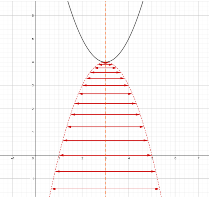
This is found on page 31 of his amazing description. His idea of ‘i-arrows’ goes far, far beyond what is necessary for simple quadratics, but it definitely can be used to demonstrate complex roots without the need for orthogonal rotation.
I love it!